 Fig.1:Schematic view of the sample setup
References:
・M. Ikebe, H. Fujishiro, T. Naito and K. Noto, Simultaneous Measurement of Thermal Diffusivity and Conductivity Applied to Bi-2223 Ceramic Superconductors, J. Phys. Soc. Jpn. 63, 3107-3114 (1994).
Fig. 1 shows a schematic view of the sample setup on the cold head of a Gifford-McMahon (GM) cycle helium refrigerator which was used as the cryostat. The attachment of both the sample to the cold-finger of the GM refrigerator and a metal film resistance heater (10kΩ) to the sample was made by use of GE7031 varnish. AuFe(0.07at.%)-Chromel thermocouples with diameter 0.076mm were used as thermometers. The temperature range for the measurement was from 4 to 300K. The sample was enclosed by a radiation shield of Ni-plated Cu which was thermally anchored to the cold head. The whole sample chamber was evacuated to 1x10⁻⁶ Torr by an oil diffusion pump. Under this experimental setup, the thermal conductivity k and thermoelectric power S were measured by a standard steady heat-flow method. An automatic measuring system was made by use of a personal computer and RS-232C and GPIB bus lines, including the GM closed cycle helium refrigerator.
Fig.1:Schematic view of the sample setup
References:
・M. Ikebe, H. Fujishiro, T. Naito and K. Noto, Simultaneous Measurement of Thermal Diffusivity and Conductivity Applied to Bi-2223 Ceramic Superconductors, J. Phys. Soc. Jpn. 63, 3107-3114 (1994).
When a heat pulse is transmitted from a heater into a sample of long and slender shape as shown in Fig.1, the time variation of temperature T(x,t) is described by the one dimensional diffusion equation,
∂T/∂t=α(∂2T/∂x2)・・・・・・ (1)
where t is the time and x is the space coordinate. This equation can be numerically solved by the Crank-Nicolson implicit method. The t-axis and the x-axis are divided by the respective unit of Δt and Δx to define discrete "lattice points" u[i,j]. Then eq. (1) is transformed to approximate difference equations given by
(1+A)u[i,j+1]-A(u[i-1,j-1]+u[i+1,j+1])/2
=(1-A)u[i,j]+A(u[i-1,j]+u[i+1,j])/2 ,・・・・・・・・ (2)
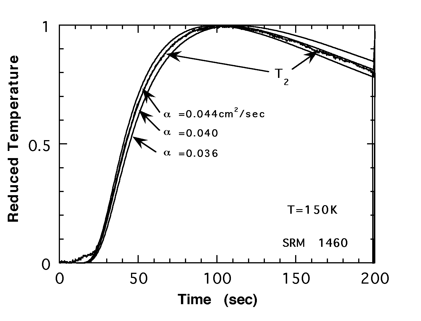
where A is a kind of the normalized diffusivity and equal to αΔt/(Δx)2. By applying a boundary condition to eq. (2), eq. (1) is finally converted into n-dimensional linear equations, which can be solved by the Gauss elimination method. We calculated the temperature change T(x,t) at arbitrary x and t with the time division Δt=0.32sec and the space division Δx=0.5mm for various values of α. The calculation was performed by a personal computer on a FORTRAN program. In the experiment, a current pulse of width 3 ~ 5 seconds was applied and the T1(t) and T2(t) were recorded for 3.1 times a second in the time span of 100 ~ 200 seconds. Then T1(t) at the point P1 is used for the boundary condition to the diffusion equation for T2(t) at the point P2. The use of the experimentally measured T1(t) as the boundary condition resolves the ambiguity due to the heat capacity of the heater and due to the various heat resistance between the heater and the sample surface.
Fig. 2 shows an example of T1(t) and T2(t) for stainless steel after impression of the current pulse at 150K. Fig. 3 shows an example of a fitting of the measured T2(t) and the calculated T2'(t). For systematic determination of α values, the maximum values of the measured and the calculated T2(t) were normalized to 1 and eighty points between 10% and 90% of the rising curve of T2(t) were sampled to give the minimum square time error Δt2 as shown in Fig. 4. This method of the diffusivity measurement had been confirmed to have about 1.5% precision and about 5% accuracy for a variety of specimens with various α values.
leftFig,2:An example of T1(t) and T2(t) (Stainless Steel): rightFig.3: Fitting of the measured T2(t) and the calculated T2'(t)

Our group joins in the Joint-research Project for Regional Intensive in the Iwate Prefecture on "Development of practical applications of magnetic field technology for use in the region and in everyday living" supported by Japan Science and Technology Corporation from 2000. In this project, we have fabricated the measuring station for the thermal properties (thermal conductivity, thermal diffusivity, specific heat, sound velocity, thermoelectric power and thermal dilatation) at the temperature range 4~400K. The magnetic field of up to 10 T was applied using a cryocooler-cooled superconducting magnet. We aim at the construction of the database of the thermal properties.
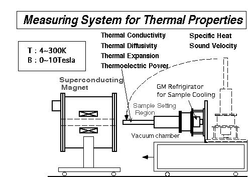
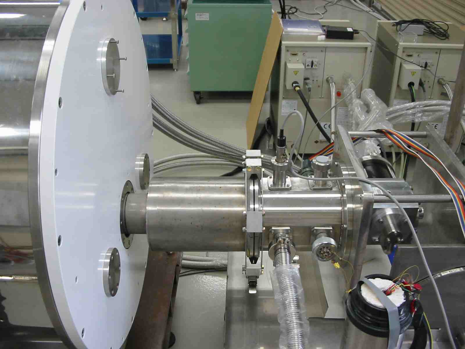
Fig.5:Apparatus under the Magnetic Field
In the field of the cryogenic engineering and low temperature physics, the thermal contact resistance (TCR) through the connection between two materials is an important parameter. For applications of high-Tc superconductors as power current leads to a cryocooled superconducting magnet (SCM), for example, it is necessary to electrically connect a high-Tc superconductor with copper leads. In such a case, TCR between them is as important as the thermal conductivity of the high-Tc superconductor itself to estimate the amount and velocity of the heat intrusion in order to avoid the quenching of SCM.
In case of applying a standard non-steady state heat flow techniques for the thermal diffusivity a measurement, the TCRs between the thermometer and the sample and between the sample and the heat sink seriously damage the accuracy of the measurements. In this case, TCR results in the time lag of temperature change T(t) of the sample and the determined a tends to be estimated lower than the true one.
The thermal contact resistance is defined by Rc=ΔT/Q [K/W], where ΔT is the discontinuous temperature difference at the interface of the two materials and Q is the heat power passing through the interface. The thermal contact resistivity Wc can be defined by Wc=RcS [mm2K/W], where S is the contact area. Even if the two materials are connected using a specified adhesive, the Wc(T) value cannot be decided uniquely because Wc(T) depends on the surface roughness of the interface, the thickness of the adhesive, the mechanical pressure in the connection and so on. Wc increases with decreasing temperature and is usually very small at the room temperature. Therefore, there is not so much investigation concerning Wc(T) except for the Kapitza resistance at very low temperatures.
We developed the measuring technique for the thermal contact resistivity Wc by steady state method and non-steady state method between 10 K and 200K and measured Wc for several connecting methods.
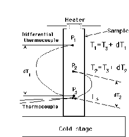
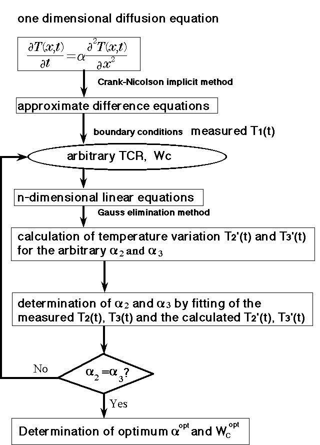
Fig.6:Schematic diagram of the experimental setup for three terminal method: Fig.7:Flow chart of the estimation of Wc
Fig. 8 shows an experimental setup around the sample for the determination of Wc. The sample (YBa2Cu3O7 polycrystal) and the copper block, both of which were situated on the cold stage of the GM cycle helium refrigerator, were connected using various adhesives (silver paste (DUPONT 4922N), In solder (99.9999% purity), epoxy resin (Stycast: 2850-GT) and varnish (GE-7031)). AuFe(0.07at.%)-chromel thermocouples with 0.076 mm in diameter were used to monitor the temperatures at P1, P2 and P3 which were attached using the silver paste. With the continuous heat power Q applied to the slender sample, the temperature jump ΔT at the interface was estimated by the extrapolation from the temperature rises at P1, P2 and P3 in the steady state.
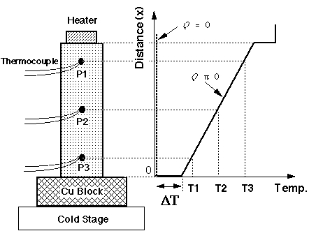
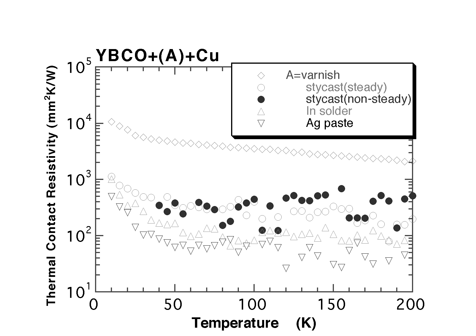
Fig.8:Experimental setup for the steady sstate method of Wc:Fig.9:Wc(T) between YBCO and Cu for various connecting methods
References:
・H. Fujishiro, M. Ikebe, K. Nakasato and T. Naito, "Proposal of Three Terminal Method for Low Temperature Thermal Diffusivity Measurement", Czech. J. Phys. 46 Suppl. S5, pp.2761-2762, 1996.
・H. Fujishiro, T. Okamoto and K. Hirose, "Thermal contact resistance between high-Tc superconductor and copper", Physica C357-360, pp.785-788, 2001
In the field of low temperature physics and cryogenic engineering, many structurally anisotropic materials (e.g.; a single crystal of high-Tc superconductors, fiber reinforced plastics (FRPs)) are used as functional and constructive materials. It is very important to investigate their anisotropic natures in mechanical, electrical and thermal transport properties. The thermal conductivity k(T) is usually measured by a one-dimensional (1D) steady-state heat flow method using a long shaped sample. For anisotropic materials, anisotropic k values (e.g.; kx, ky, kz) are measured in separate experimental setups using long shaped samples cut along an each direction.
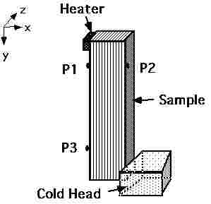 Fig.10:Experimental setup for 2D analyses
References:
・H. Fujishiro, T. Okamoto,M. Ikebe and K. Hirose "A New Method for Simultaneous Determination of Anisotropic Thermal Conductivities Based on Two-dimensional Analyses", Jpn. J. Appl. Phys. 40, pp.388-392, 2000
・H. Fujishiro, M. Ikebe, K. Nakasato and T. Naito, "Proposal of Three Terminal Method for Low Temperature Thermal Diffusivity Measurement", Czech. J. Phys. 46 Suppl. S5, pp.2761-2762, 1996